Short Course
Regularised Estimation Procedures in Spatiotemporal Statistics
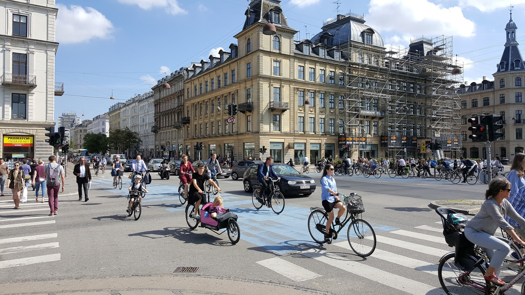
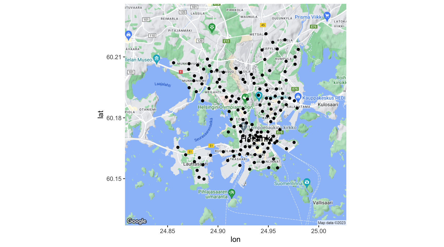
Cyclists in the city centre of Helsinki (https://ecf.com/news-and-events/news/visionarycities-series-will-helsinki-be-next-cycling-capital)
# time lag k = 1, ...
k <- 1

plot(avg_bikes[-c(1:k)], avg_bikes[-c((length(avg_bikes)-k+1):length(avg_bikes))],
       col = color_vector[-c(1:k)],
       xlab = "Average number of bikes per station",
       ylab = "Average number of bikes per station 5 minutes ago",
       axes = FALSE)
  axis(1, seq(0, 10, by = 0.5))
  axis(2, seq(0, 20, by = 0.5))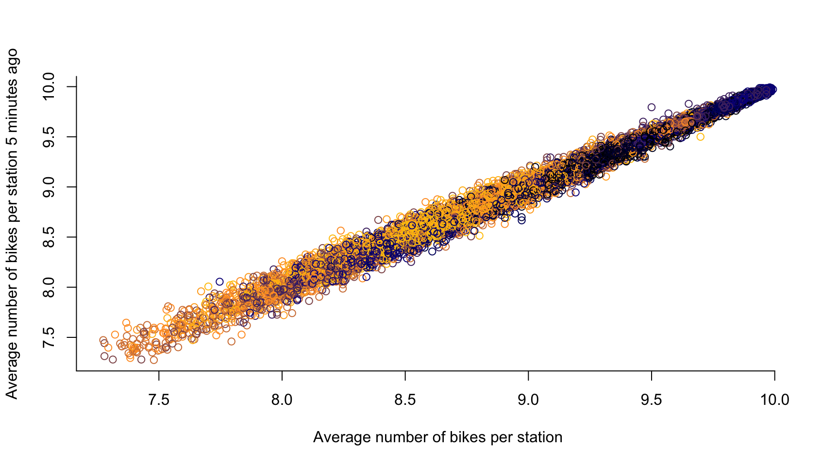
# time lag k = 1, ...
k <- 2

plot(avg_bikes[-c(1:k)], avg_bikes[-c((length(avg_bikes)-k+1):length(avg_bikes))],
       col = color_vector[-c(1:k)],
       xlab = "Average number of bikes per station",
       ylab = "Average number of bikes per station 10 minutes ago",
       axes = FALSE)
  axis(1, seq(0, 10, by = 0.5))
  axis(2, seq(0, 20, by = 0.5))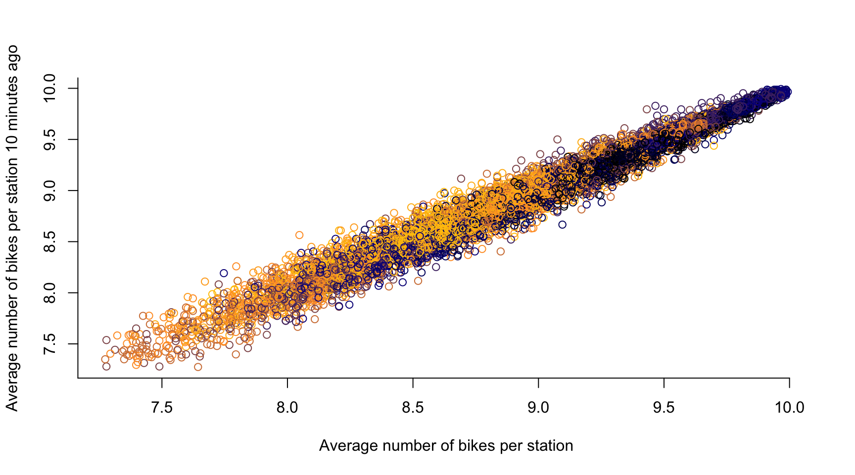
# time lag k = 1, ...
k <- 3

plot(avg_bikes[-c(1:k)], avg_bikes[-c((length(avg_bikes)-k+1):length(avg_bikes))],
       col = color_vector[-c(1:k)],
       xlab = "Average number of bikes per station",
       ylab = "Average number of bikes per station 15 minutes ago",
       axes = FALSE)
  axis(1, seq(0, 10, by = 0.5))
  axis(2, seq(0, 20, by = 0.5))
# time lag k = 1, ...
k <- 4

plot(avg_bikes[-c(1:k)], avg_bikes[-c((length(avg_bikes)-k+1):length(avg_bikes))],
       col = color_vector[-c(1:k)],
       xlab = "Average number of bikes per station",
       ylab = "Average number of bikes per station 20 minutes ago",
       axes = FALSE)
  axis(1, seq(0, 10, by = 0.5))
  axis(2, seq(0, 20, by = 0.5))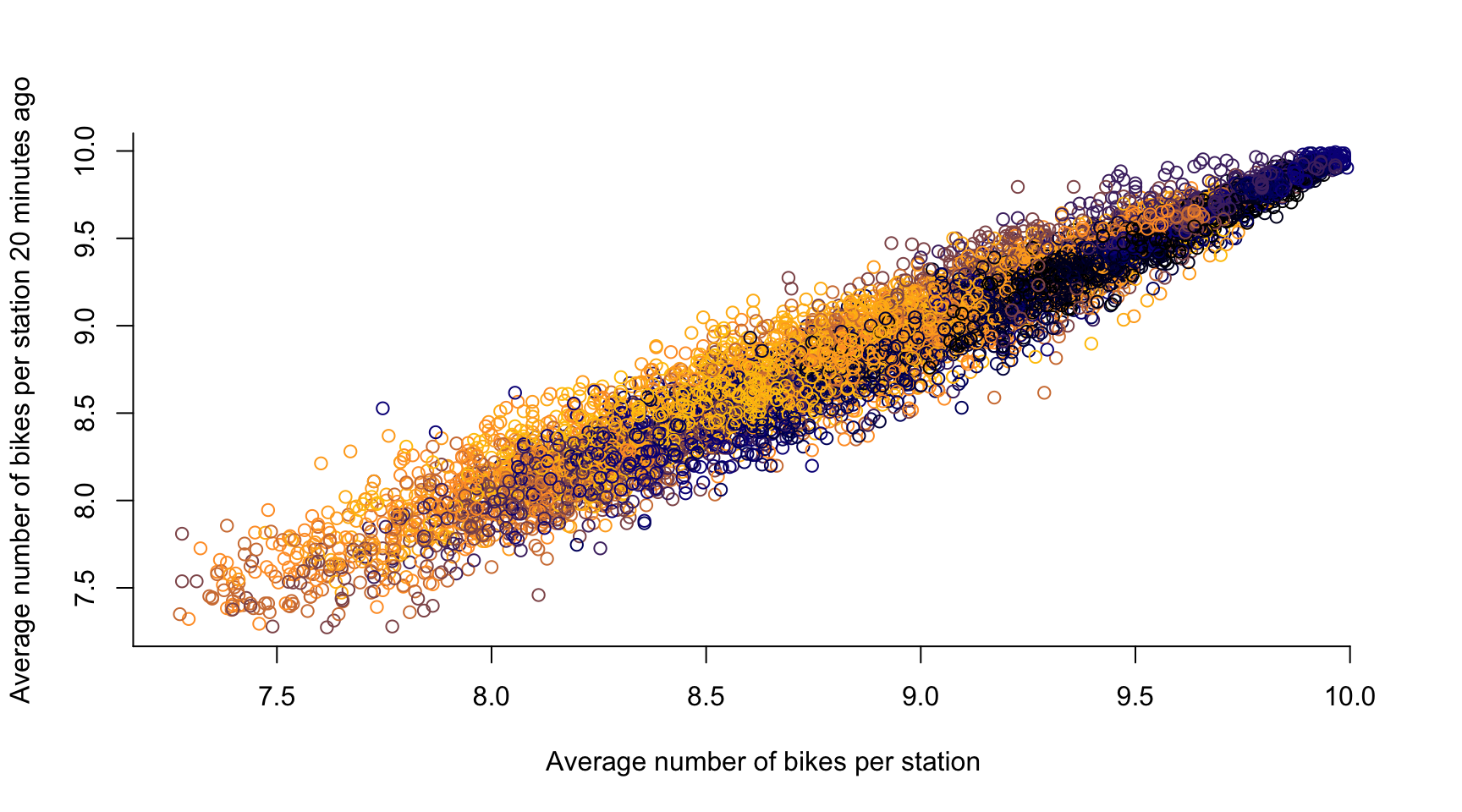
# time lag k = 1, ...
k <- 12

plot(avg_bikes[-c(1:k)], avg_bikes[-c((length(avg_bikes)-k+1):length(avg_bikes))],
       col = color_vector[-c(1:k)],
       xlab = "Average number of bikes per station",
       ylab = "Average number of bikes per station one hour ago",
       axes = FALSE)
  axis(1, seq(0, 10, by = 0.5))
  axis(2, seq(0, 20, by = 0.5))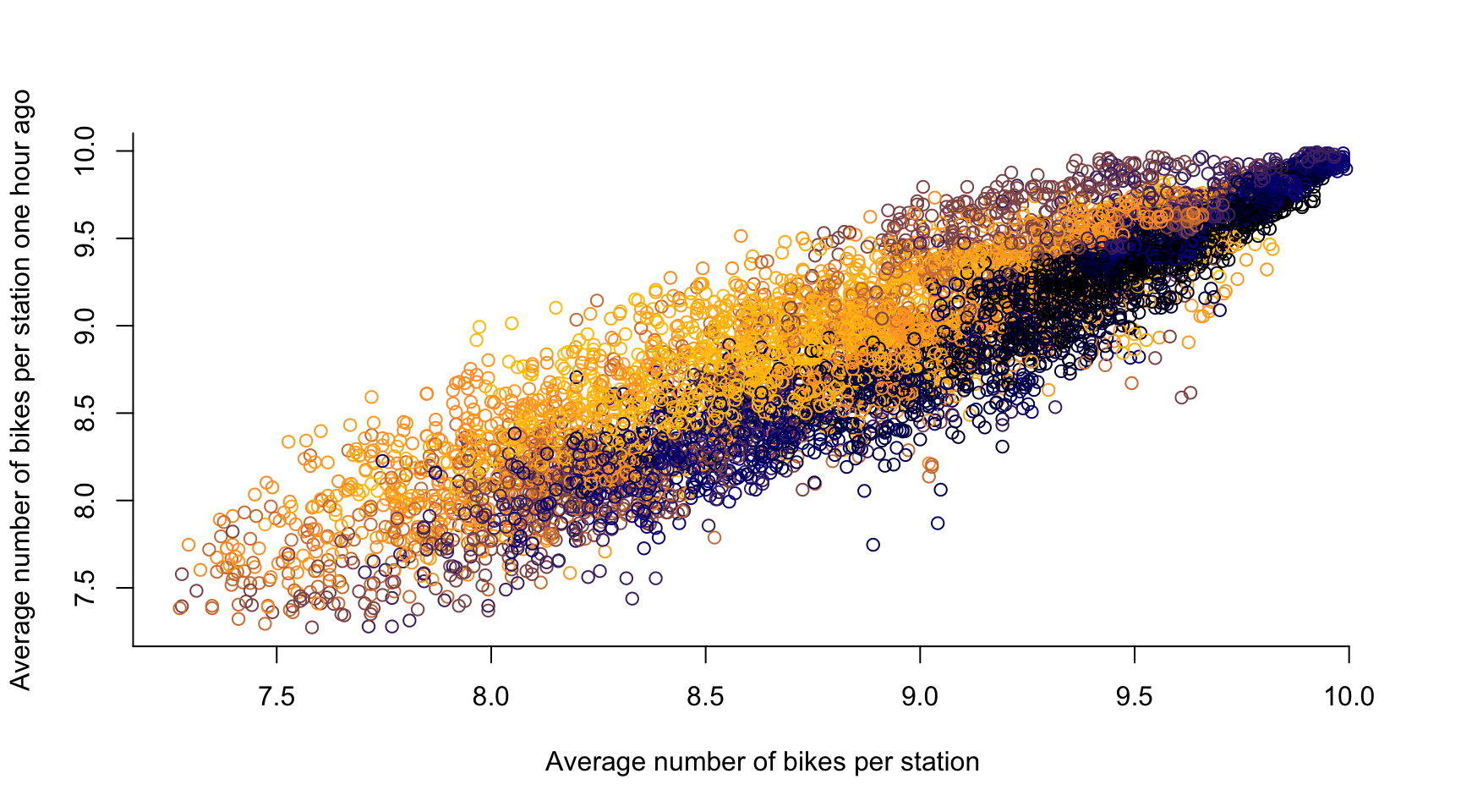
# time lag k = 1, ...
k <- 24

plot(avg_bikes[-c(1:k)], avg_bikes[-c((length(avg_bikes)-k+1):length(avg_bikes))],
       col = color_vector[-c(1:k)],
       xlab = "Average number of bikes per station",
       ylab = "Average number of bikes per station two hours ago",
       axes = FALSE)
  axis(1, seq(0, 10, by = 0.5))
  axis(2, seq(0, 20, by = 0.5))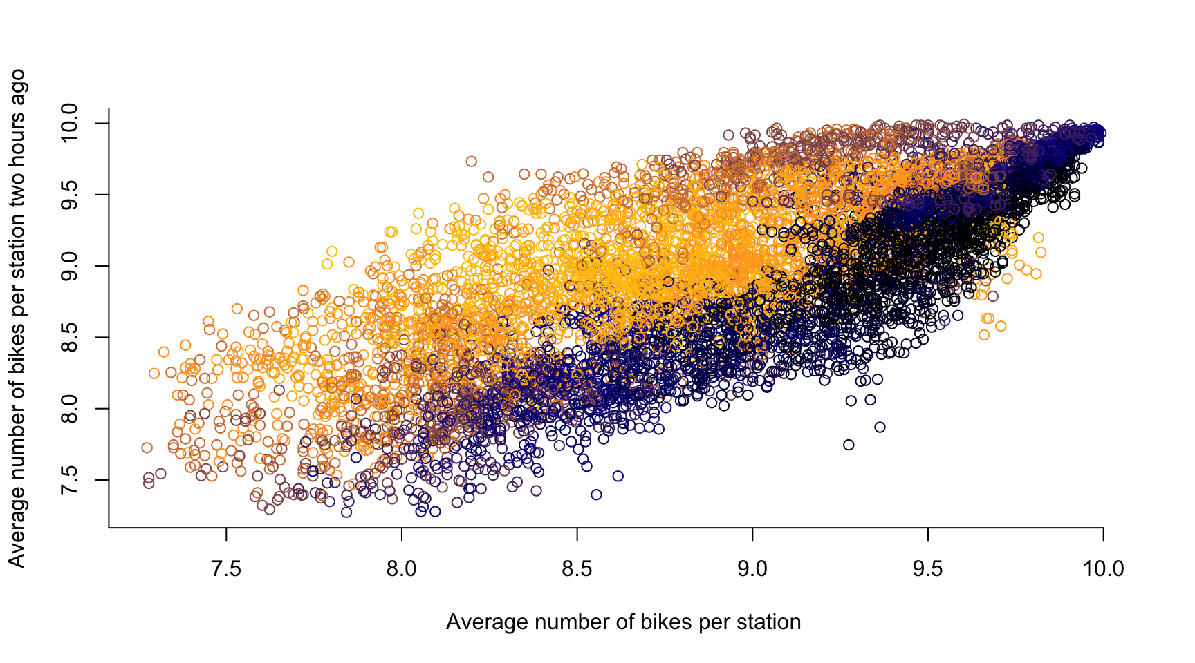
Expand for full code
Expand for full code
bikes_space <- bikes[which(months(times) == "July"), ]

k       <- 3
t       <- 1

knnW    <- t(sapply(1:n, function(i) ifelse(dist_mat[i,] < sort(dist_mat[i,])[k+2] & dist_mat[i,] > 0, 1/k, 0))) # k+2, because of the diagonal zero entry and the strict inequality
plot(bikes_space[t,],
     knnW %*% ifelse(is.na(bikes_space[t,]), mean(bikes_space[t,], na.rm = TRUE), bikes_space[t,]),
     ylim = c(0, 60),
     xlim = c(0, 60),
     ylab = "Average bike count of k-nearest neighbours",
     xlab = "Average bike count midnight",
     col = color_vector[t])

x <- knnW %*% ifelse(is.na(bikes_space[t,]), mean(bikes_space[t,], na.rm = TRUE), bikes_space[t,])
ab <- lm(bikes_space[t,] ~ x)$coeff
text(50, 50, ab[2])
abline(a = ab[1], b = ab[2])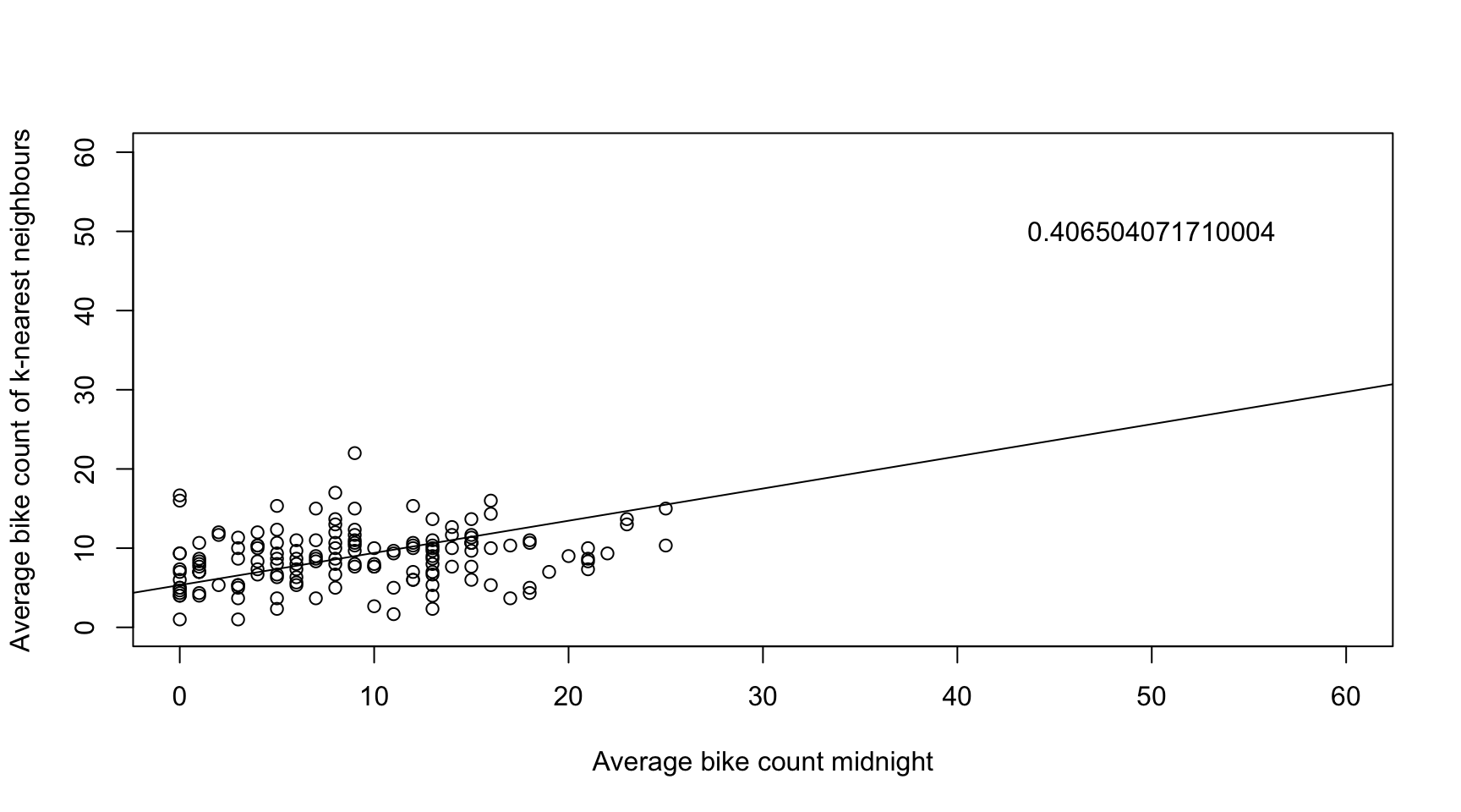
h <- 1 # index time point across the day

plot(1:100, M.I,
      col = colors[h],
      main = paste("Spatial Correlation (Moran's I) at ", h-1, ":00", sep = ""),
      pch = ifelse(M.Ip < 0.05, 20, 1),
      ylim = c(0, 0.8),
      axes = FALSE,
      xlab = "Spatial lag order (k-nearest neighbours)",
      ylab = "Spatial correlation (Moran's I)")
axis(1, seq(-20, 120, by = 10))
axis(2, seq(-1, 1, by = 0.05))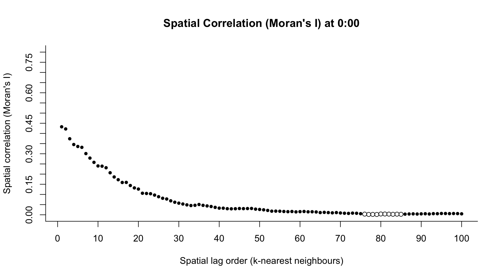
h <- 8 # index time point across the day

plot(1:100, M.I,
      col = colors[h],
      main = paste("Spatial Correlation (Moran's I) at ", h-1, ":00", sep = ""),
      pch = ifelse(M.Ip < 0.05, 20, 1),
      ylim = c(0, 0.8),
      axes = FALSE,
      xlab = "Spatial lag order (k-nearest neighbours)",
      ylab = "Spatial correlation (Moran's I)")
axis(1, seq(-20, 120, by = 10))
axis(2, seq(-1, 1, by = 0.05))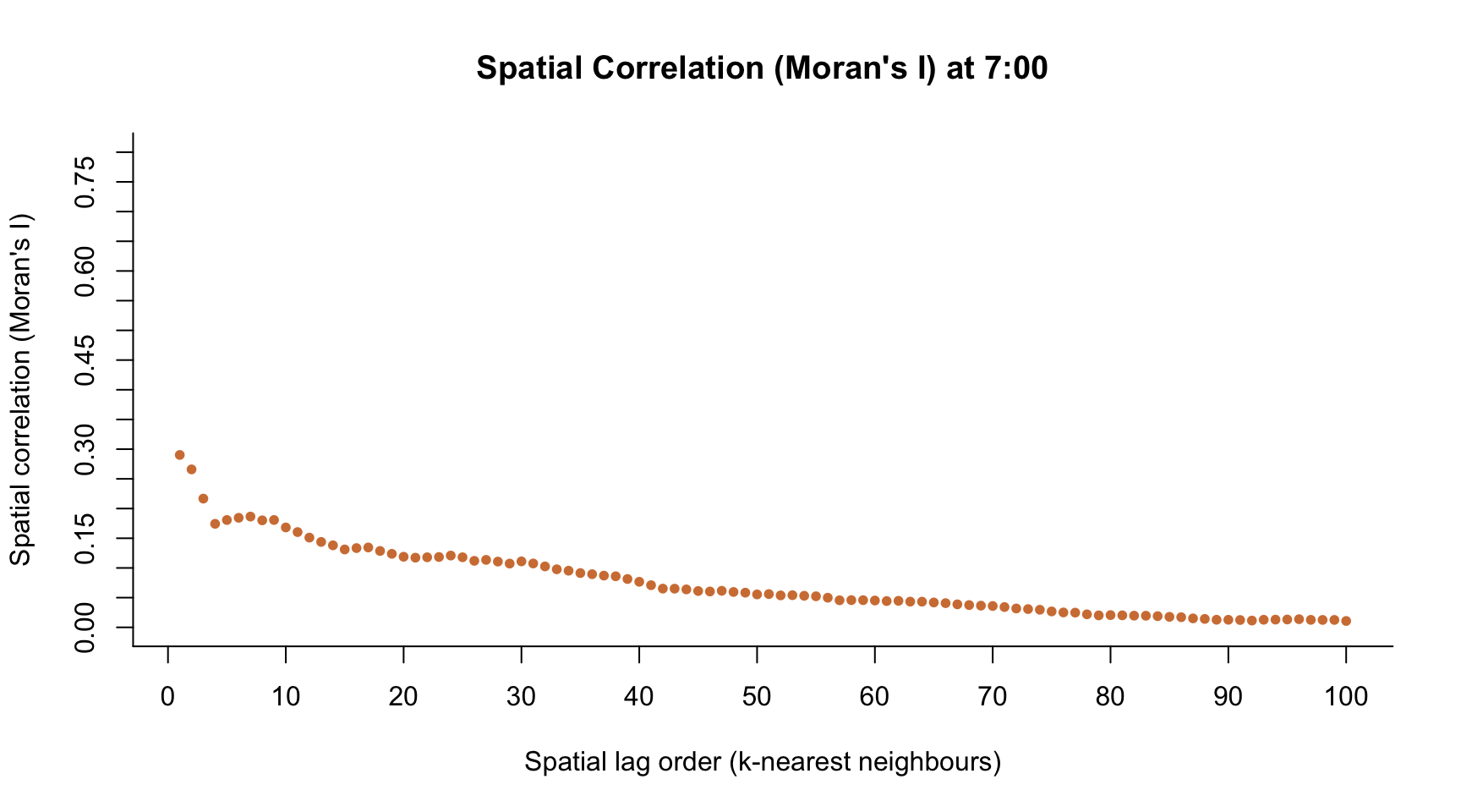
h <- 13 # index time point across the day

plot(1:100, M.I,
      col = colors[h],
      main = paste("Spatial Correlation (Moran's I) at ", h-1, ":00", sep = ""),
      pch = ifelse(M.Ip < 0.05, 20, 1),
      ylim = c(0, 0.8),
      axes = FALSE,
      xlab = "Spatial lag order (k-nearest neighbours)",
      ylab = "Spatial correlation (Moran's I)")
axis(1, seq(-20, 120, by = 10))
axis(2, seq(-1, 1, by = 0.05))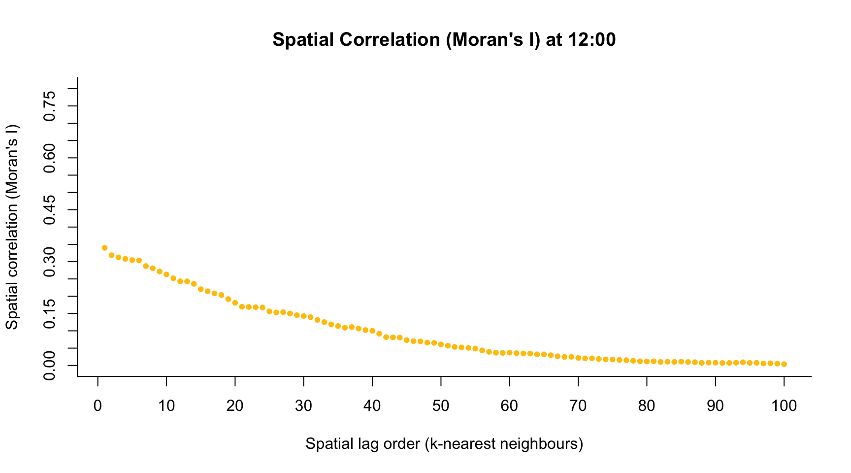
load("sources/data_berlin.rda")
library("maptools")
library("spdep")

B <- data_berlin$map
IDs <- as.character(names(B))
n <- length(unique(IDs))

plot(B)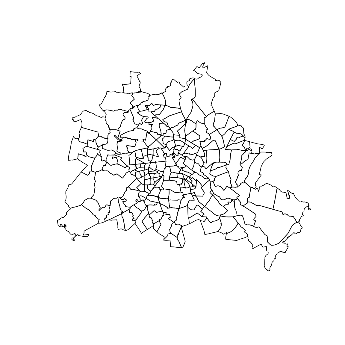
IDs4 <- substr(as.character(names(B)), 1, 4)
n_thin <- length(unique(IDs4))

if(!gpclibPermitStatus()){
  gpclibPermit()
}
[1] TRUEB_thin <- unionSpatialPolygons(B, IDs4)
coords <- array(, dim = c(length(B), 2))
for(i in 1:length(B)){
coords[i,] <- B@polygons[[i]]@labpt
}
cols <- colorRampPalette(c("white", "darkblue"))
# Inverse-distance matrix
W <- 1 / as.matrix(dist(coords))
diag(W) <- 0
image(1:n, 1:n, W, col = cols(10))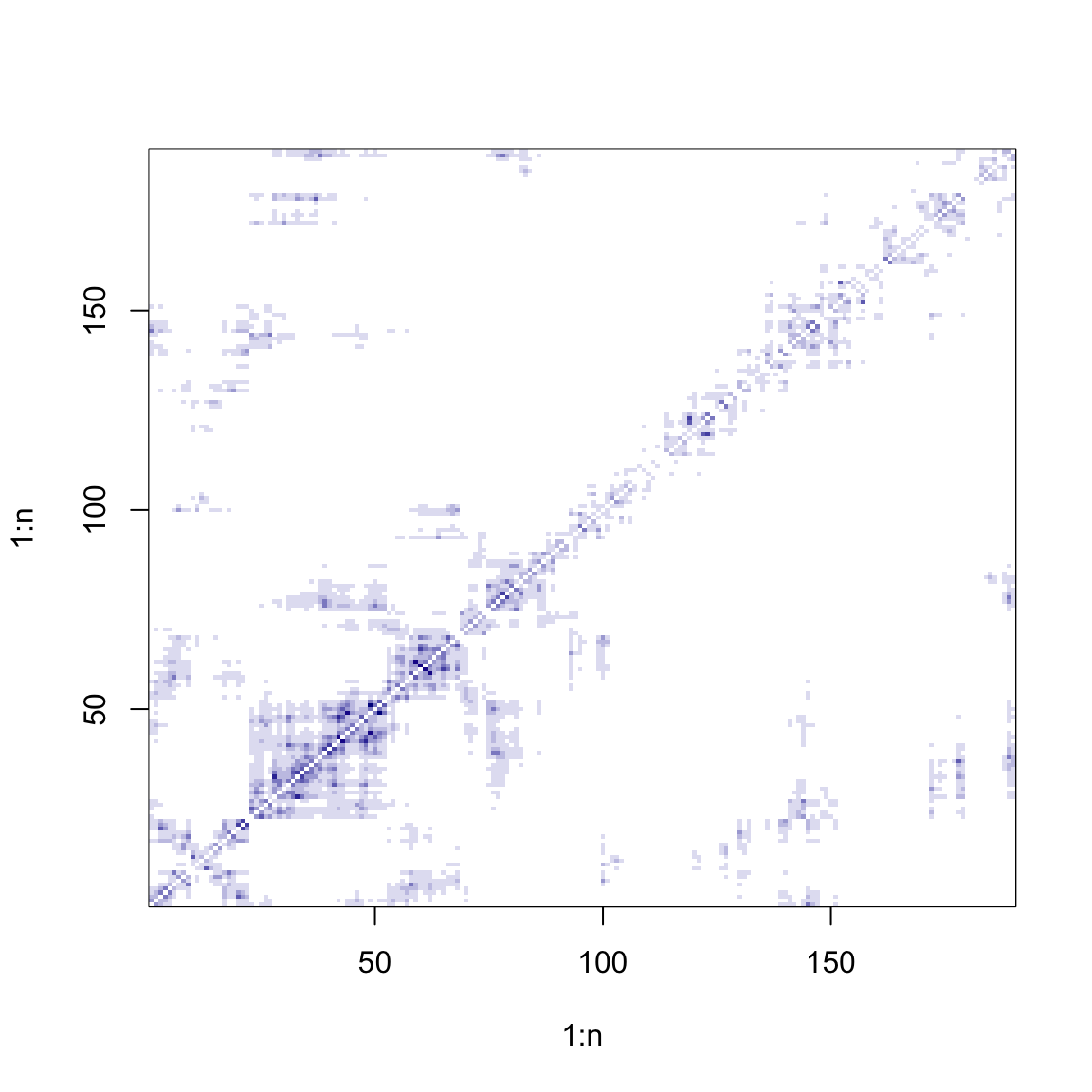
# Inverse-distance matrix (row-standardised)
W <- W / array(apply(W, 1, sum), dim = dim(W))
image(1:n, 1:n, W, col = cols(10))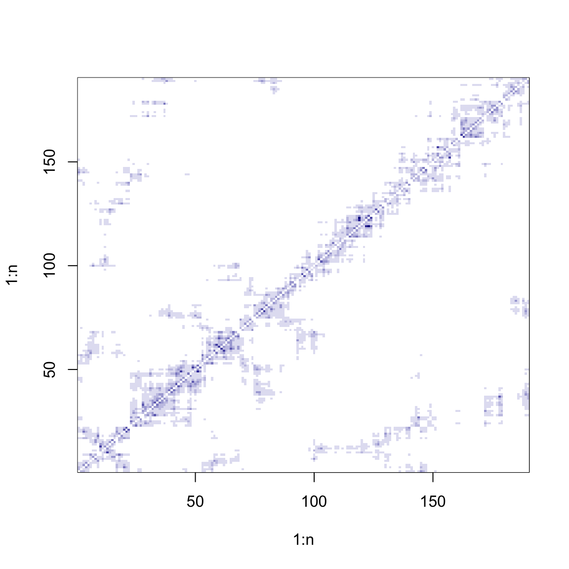
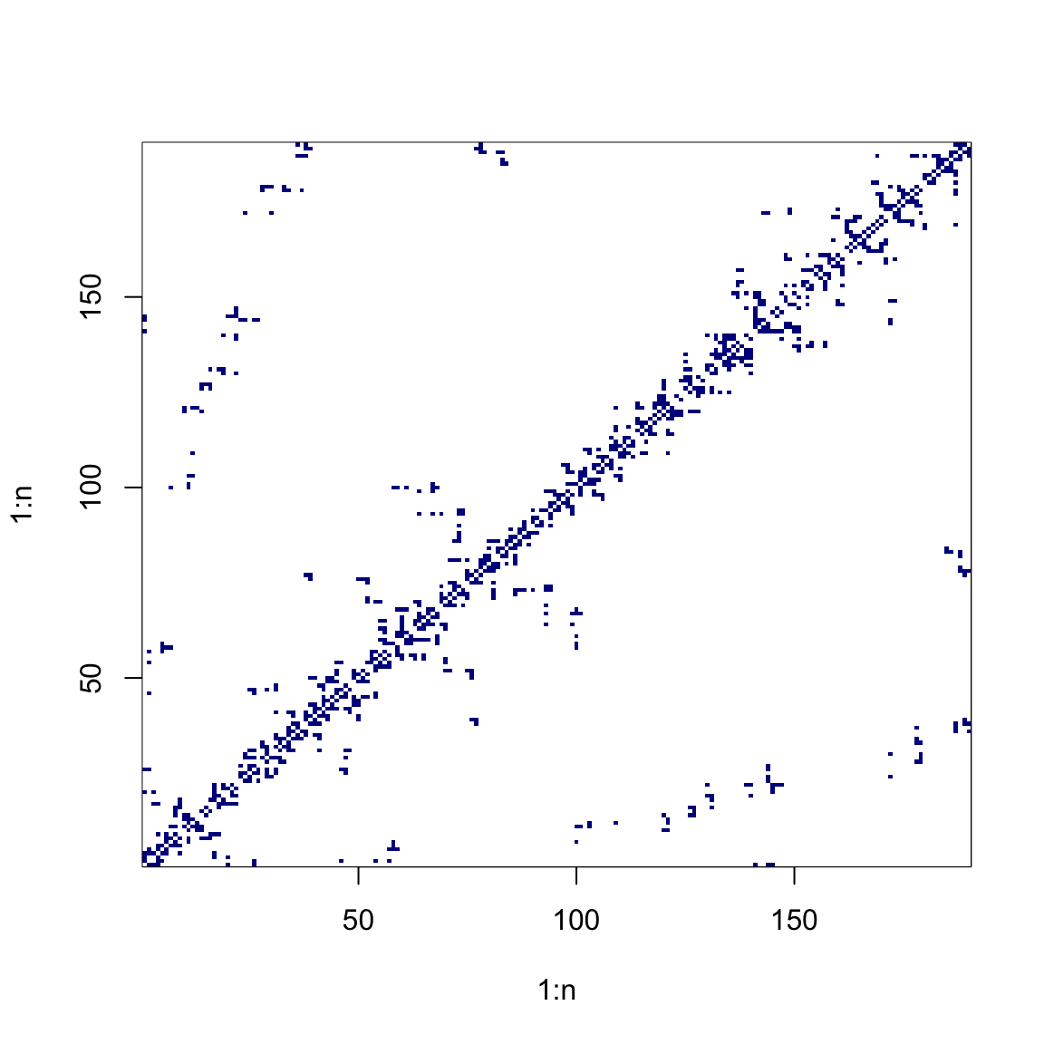
# Contiguity matrix (row-standardised)
W <- nb2mat(poly2nb(B), style = "W")
image(1:n, 1:n, W, col = cols(10))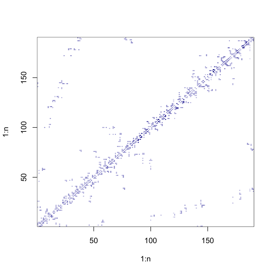
W_list <- poly2nb(B)
plot(B, border = "lightgrey")
plot(B_thin, add = TRUE, lwd = 1)
plot(W_list, coordinates(B), pch = 1, add = TRUE, col = "darkblue",
     lwd = 2, # 10*apply(W, 1, max),
     cex = 0.2*apply(W, 2, function(x) sum(x>0)))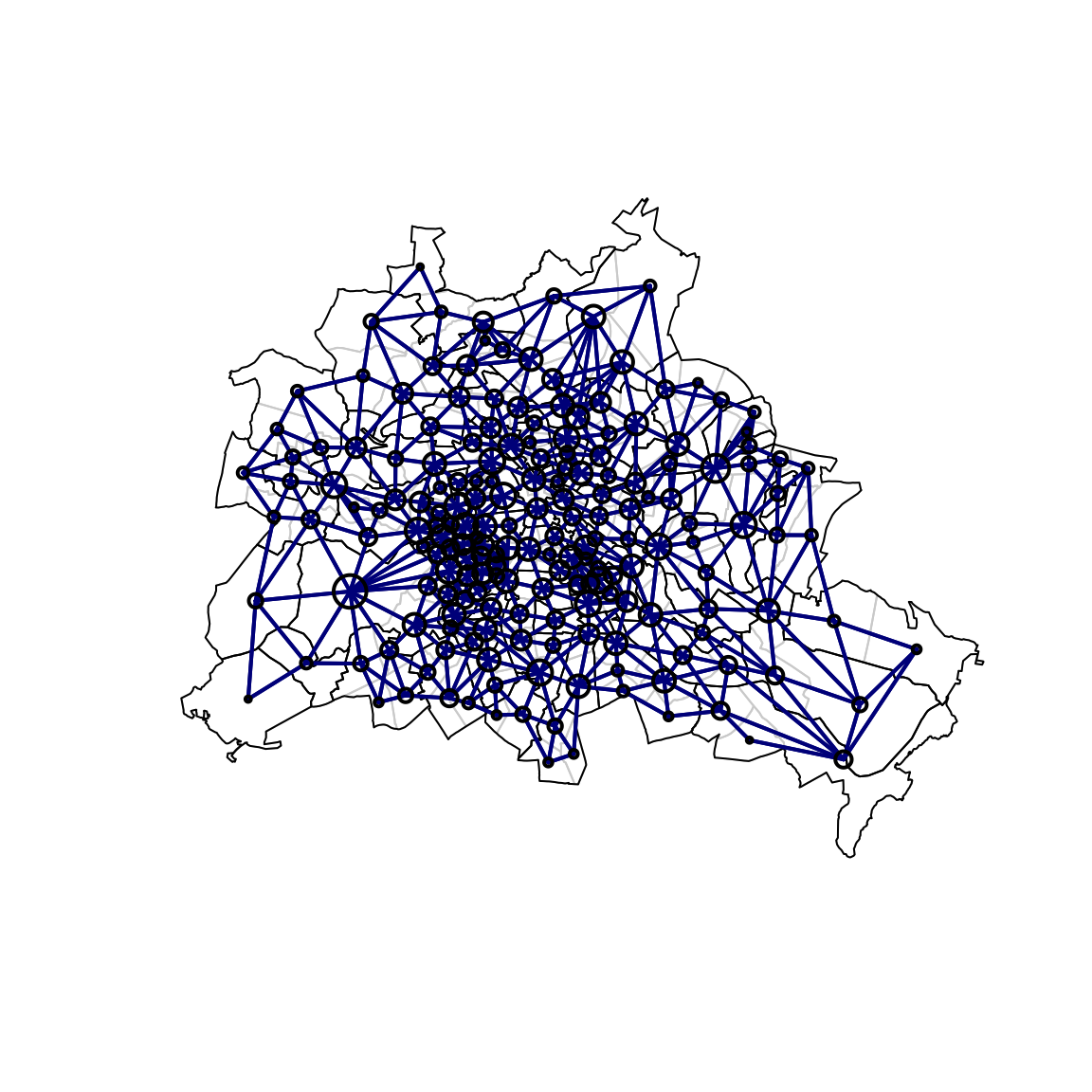
Implementation in R
Implementation in Python
# Load the required libraries
from sklearn.linear_model import lasso_path
import matplotlib.pyplot as plt
import numpy as np
import pandas as pd
from itertools import cycle

# Load the sample data
cars = pd.read_csv('sources/mtcars.csv', index_col = 0, header = 0)

lambdas = np.logspace(-4.5, 0.9, 100)

# Split the data into features and target
X = cars.drop('mpg', axis=1)
y = cars['mpg']

# Standardize data
X -= X.mean(axis=0)
X /= X.std(axis=0)

# Use lasso_path to compute a coefficient path
alphas_lasso, coef_path, _ = lasso_path(X, y, alphas = lambdas)

# Plot coefficients against lambda
plt.figure();
colors = cycle(["b", "r", "g", "c", "k"])
for coefs, c in zip(coef_path, colors):
    l1 = plt.plot(alphas_lasso, coefs, c = c);
plt.xlabel("Log Lambda");
plt.ylabel("Coefficients");
plt.xscale('log');
plt.title("Lasso Coefficient Path");
plt.axis("tight");

plt.show()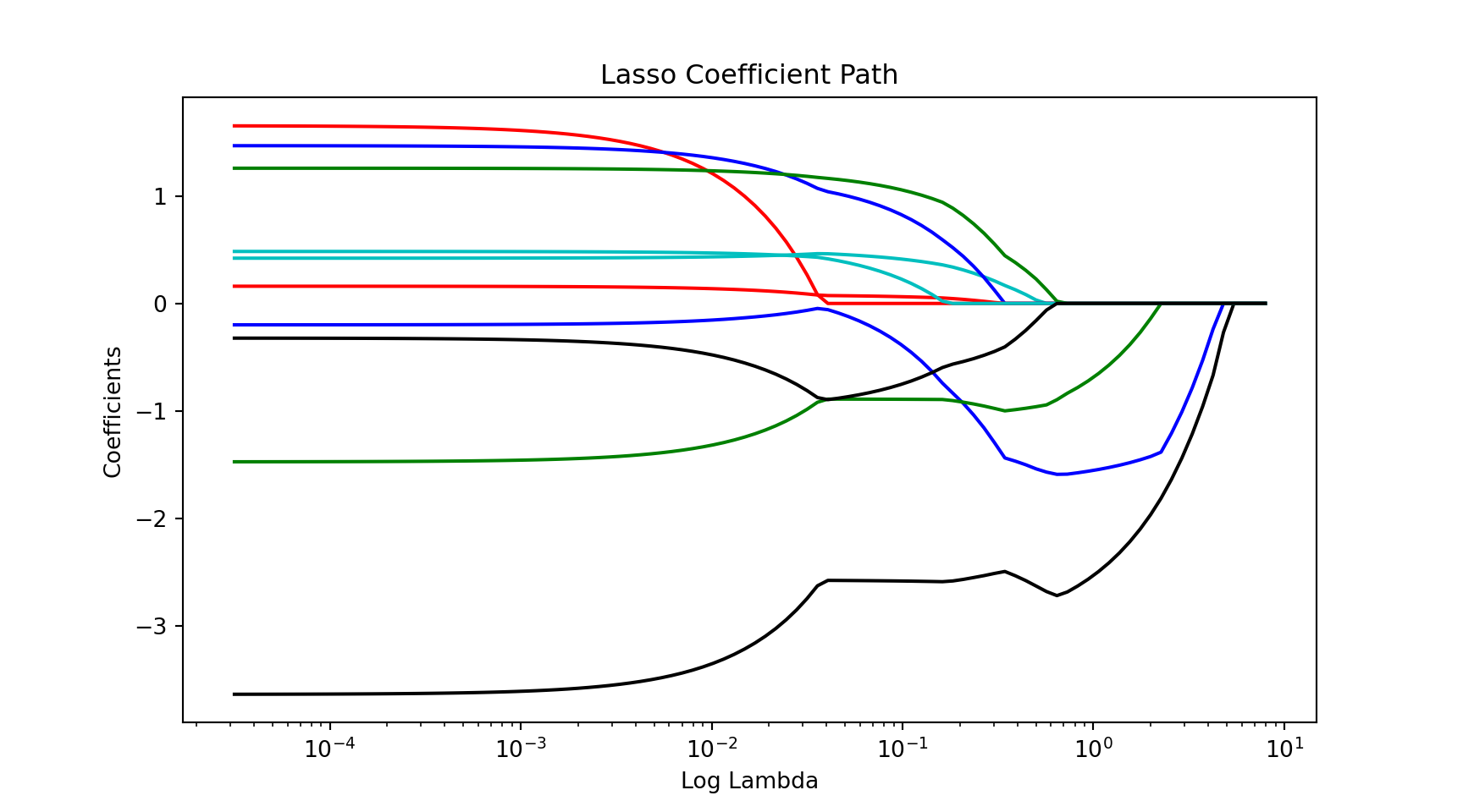
3.4 Elastic Net
Convex combination of both penalties: \[\begin{equation*} \hat{\boldsymbol{\beta}} = \arg \min_{\boldsymbol{\beta} \in \mathbb{R}^{p}} \frac{1}{n} (\boldsymbol{Y} - \mathbf{X} \, \boldsymbol{\beta})^\prime (\boldsymbol{Y} - \mathbf{X} \, \boldsymbol{\beta}) + \lambda_1 ||\beta||_1 + \lambda_2 ||\beta||_2 \end{equation*}\] with regularisation parameter \(\lambda \geq 0\).
- Grid-search over two-dimensional space \((\lambda_1, \lambda_2)'\)
- If \(\lambda_1 \rightarrow 0\), the \(\hat{\boldsymbol{\beta}}(\lambda_1, \lambda_2) \rightarrow \hat{\boldsymbol{\beta}}_{\text{Ridge}}(\lambda_2)\)
- If \(\lambda_2 \rightarrow 0\), the \(\hat{\boldsymbol{\beta}}(\lambda_1, \lambda_2) \rightarrow \hat{\boldsymbol{\beta}}_{\text{Lasso}}(\lambda_1)\)
- Elastic nets can be reduced to the linear support vector machine (i.e., SVM solvers can be applied)
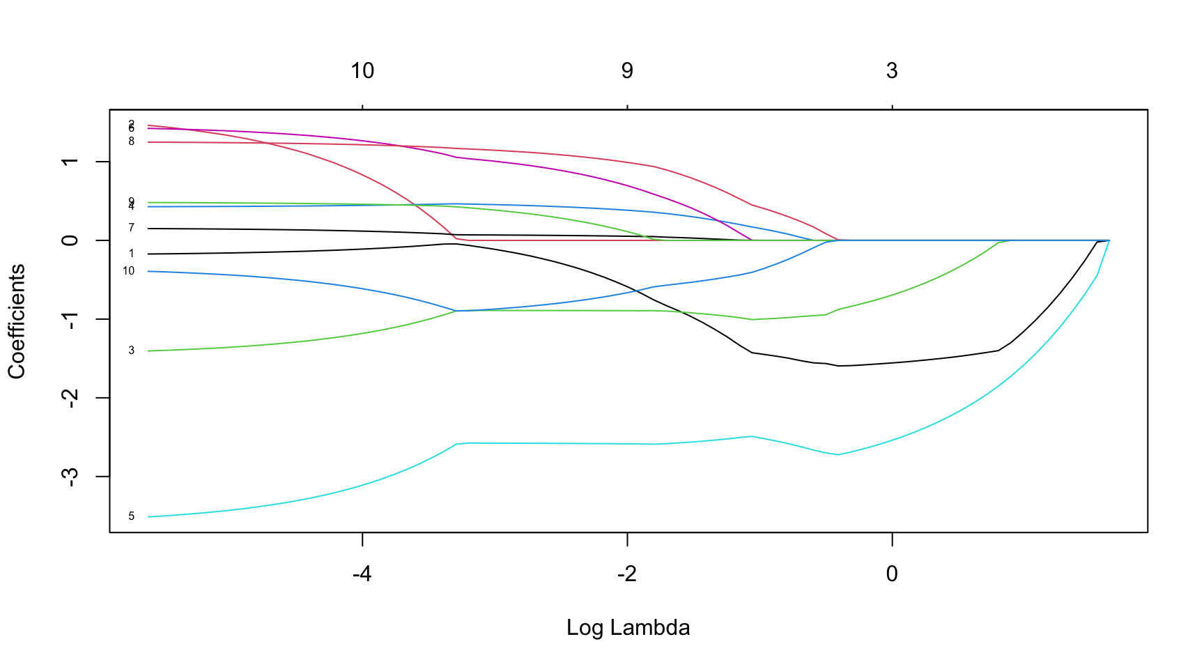
library(glmnet)

# Load the sample data
data(mtcars)

# Convert the data to matrices
X <- as.matrix(mtcars[, -1])
y <- as.matrix(mtcars[, 1])

X <- scale(X)

# Fit the LASSO model
fit <- glmnet(X, y, intercept = TRUE, alpha = 0.5)
# alpha elastic net mixing parameter

# Plot the lambda path
plot(fit, xvar = "lambda", label = TRUE)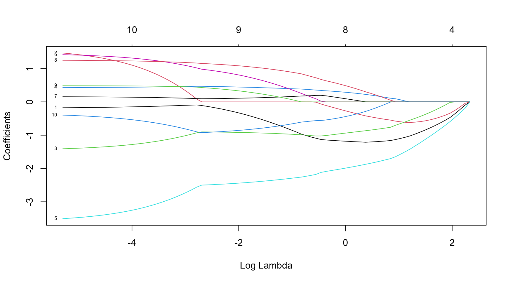
# Load the required libraries
from sklearn.linear_model import LassoCV
import matplotlib.pyplot as plt
import numpy as np
import pandas as pd
# Load the sample data
cars = pd.read_csv('sources/mtcars.csv', index_col = 0, header = 0)
lambdas = np.logspace(-4.5, 0.9, 100)
# Split the data into features and target
X = cars.drop('mpg', axis=1)
y = cars['mpg']
# Standardize data
X -= X.mean(axis=0)
X /= X.std(axis=0)
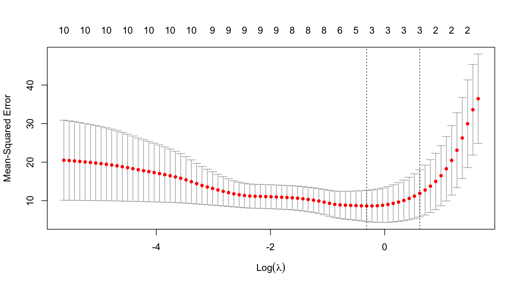
# Fit LASSO model with cross-validation and k = 10 folds
model = LassoCV(alphas = lambdas, cv = 10).fit(X, y);
# Plot average MAE across the lambda sequence
plt.semilogx(model.alphas_, model.mse_path_, ":");
plt.semilogx(model.alphas_, model.mse_path_.mean(axis=1), 'k',
label=r'Average across the folds', linewidth = 2);
plt.xlabel(r'$\lambda$');
plt.ylabel('Mean squared error');
plt.title('Mean squared error on each fold: Lasso');
plt.axis('tight');
plt.show()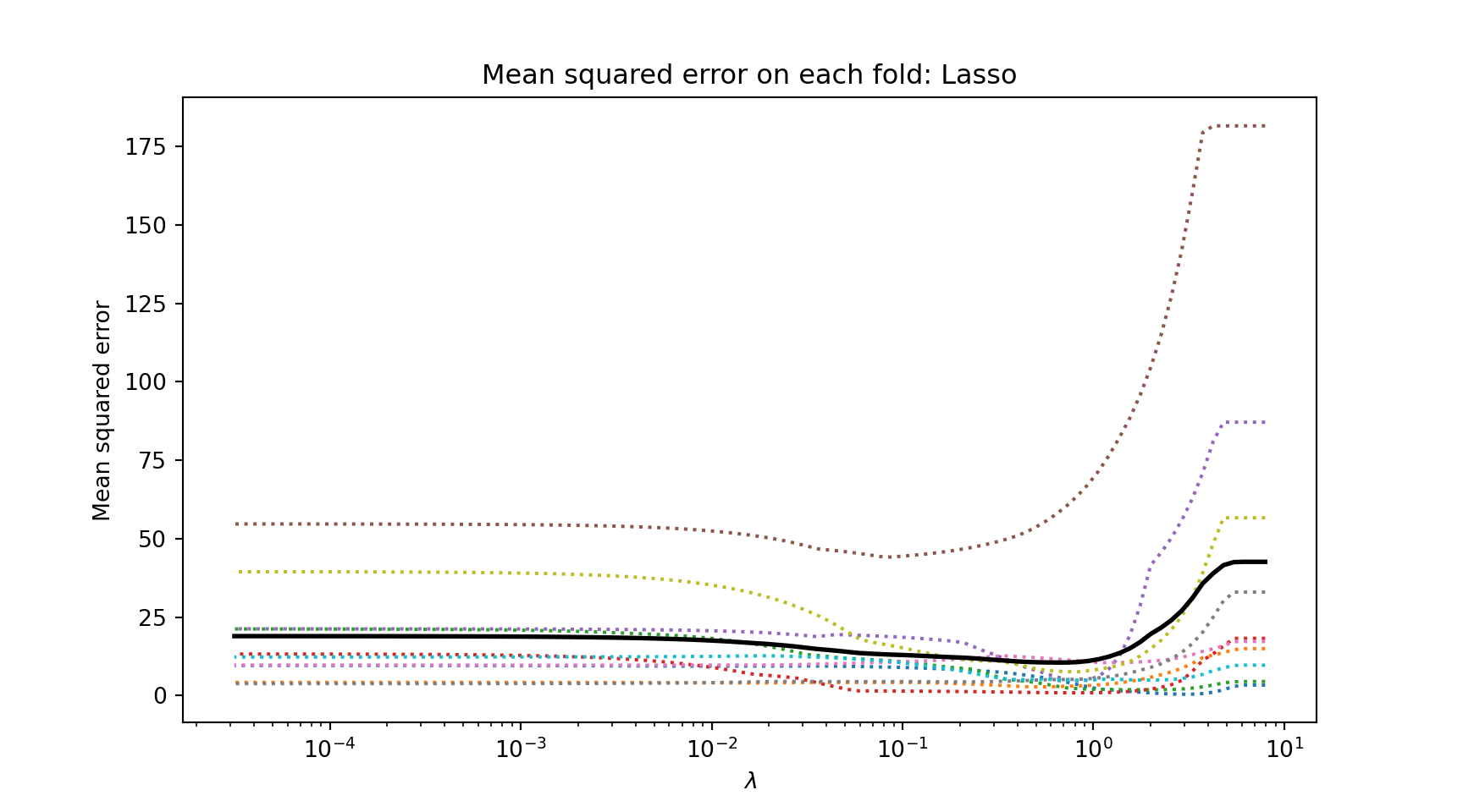
4.2 Dimensionality Reduction Covariance Matrix
- Big-\(N\) Problem \(\leadsto\) clever methods to reduce the dimensionality are needed to apply geostatistical models to large data data sets
Methods to reduce the dimensionality of the covariance matrix:
- Sparse covariance matrix (i.e., covariance matrix resulting from \(C_\theta\) contains many zeros)
- covariance tapering (Furrer, Genton, and Nychka 2006)
- theoretical results on covariance tapering can be found in Stein (2013)
- covariance tapering for likelihood-based estimation procedures (see Kaufman, Schervish, and Nychka 2008; Furrer, Bachoc, and Du 2016)
Regularised estimation procedures (with a shrinkage target of zero)
We can typically find zeros if two observations across space/time are conditionally independent, but conditional independence is encoded in the precision matrix (i.e., inverse covariance matrix):
- Lasso procedure to induce zeros in the precision matrix (see Krock, Kleiber, and Becker 2021 for univariate processes; and Krock et al. 2021 for multivariate processes)
- Graphical Lasso
library(gstat)
library(glasso)

set.seed(5515)

# Simulation of geostatistical process
xy <- expand.grid(1:10, 1:10)
names(xy) <- c("x","y")
gridded(xy) = ~x+y
g.dummy <- gstat(formula = z ~ 1, dummy = TRUE, beta = 0,  model = vgm(1, "Exp", 15), nmax = 100) # for speed -- 10 is too small!!
yy <- predict(g.dummy, xy, nsim = 500)
spplot(yy[1:10])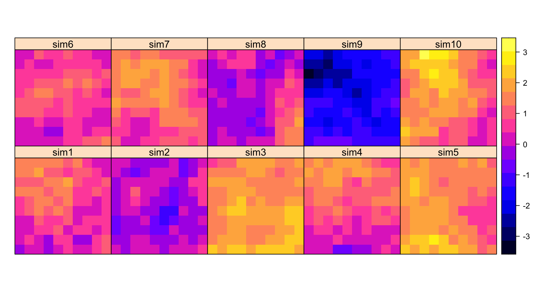
# graphical Lasso
x <- t(do.call(cbind, lapply(1:500, function(x) yy[x]@data)))
s <- var(x)
lambda.seq <- 2^seq(from = -2, to = 0.5, length = 50)
a <- glassopath(s, rholist = lambda.seq)
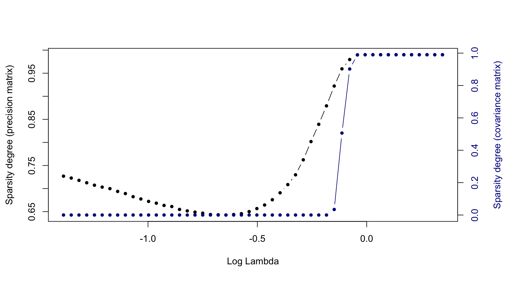
# Plot the share of zeros in the estimated precision matrix
par(mar = c(5, 4, 4, 4) + 0.3)
plot(log(a$rholist), apply(a$wi, 3, function(x) mean(x == 0)),
type = "b", pch = 20,
xlab = "Log Lambda", ylab = "Sparsity degree (precision matrix)")
par(new = TRUE)
plot(log(a$rholist), apply(a$w, 3, function(x) mean(x == 0)),
type = "b", , pch = 20, col = "darkblue", axes = FALSE, ylab = "", xlab = "")
axis(side=4, at = pretty(range(apply(a$w, 3, function(x) mean(x == 0)))), col.axis = "darkblue")
mtext("Sparsity degree (covariance matrix)", side = 4, line = 3, col = "darkblue")